6 Introduction to Graphs
6.1 The Building Blocks of Graphs: Edges and Nodes
There is a mathematical definition of a graph which is slightly more technical. A graph is a set, usually represented by the capital letter G.
From high school math, you may remember that the mathematical definition of a set is simply a collection of entities, some of which may be ordered and some of which may themselves be other sets (a set can have other sets as its members, like in the movie Inception, where you can have a dream inside a dream). In the case of graphs, the entities inside the collection are a set of vertices (also called nodes) and a separate set of edges (also called links).
A graph is thus a set containing two sets as its members: a set of nodes (usually represented by the capital letter V) and a set of edges (usually represented by the capital letter E).
In set theory notation:
\[ G = \{V, E\} \tag{6.1}\]
This says that the members of the set defined by the graph, which we call G, are two other sets, called E and V (which themselves have members). The usual notation, like in Equation eq-graph, is to enclose the members of a set in brackets \(\{\}\).
6.1.1 Nodes
The set of nodes usually represents actors in the real-world social network. Point and line diagrams (such as the ones shown in sec-tiesbound) are used to represent graphs, which in turn represent the real social network.
In these diagrams, nodes (representing actors) are usually drawn as circles, but they can be any shape or symbol. In social network analysis, actors are often either an individual or an organization, but, as we have seen, in wider applications of the network imagery in the physical and biological sciences (usually going under the banner of network science), nodes can represent anything that links up to other similar entities in a larger system. These include power generation stations and homes, servers and computers, animals in an ecosystem, towns, really anything of substance that we can define some kind of relation on, or from which some type of content can be said to be exchanged.
6.1.2 Edges
Edges represent a connection or a social tie between two nodes. As we will see, this can be a permanent relationship (e.g., “brother of”) or a more fleeting interaction (e.g., a text message, being in the same place at the same time). We will define social ties, how many types exist, and their properties later. For now, we can say that in social network analysis, connections are relationships, or links between nodes, and edges in a graph are meant to represent these connections.
In graph theory, the set of edges is best thought of as a collection of pairs of nodes, where the two members of the pair are the nodes involved in the social tie. So if node A is linked to node B via some social tie (friendship, study group, coworkers), then AB is a member of the edge set of the relevant graph. In set theory notation, this is usually written as \(AB \in E\), which is read as “the edge AB is a member of the set \(E\).” Edges can also be referred to by juxtaposing the two nodes that are connected by the edge. Thus, the edge AB can also be written as \(V_A V_B\).
In the case of power generation stations and homes, the edges can represent power lines. Meanwhile, servers and computers are connected via internet cables and Wi-Fi, while towns are connected by roads. The existence of edges signals the potential for content to flow, whether that’s power, computer data, or people in cars. In social networks, the content that flows between two nodes includes influence, advice, information, and support. All of these things are either positive or neutral, but the content that flows through social ties can also be negative, like a disease, bullying, gossip, or even murder (e.g., between rival gangs).
6.2 What is a Graph?
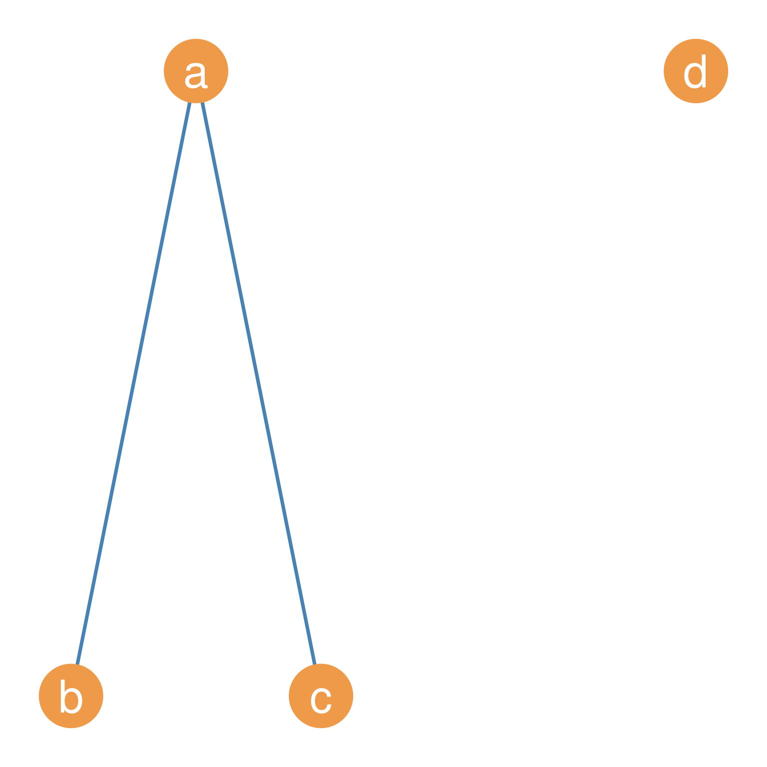
Figure fig-simple-1 shows an example of a point and line network diagram of a graph with four nodes and two edges. Nodes A, B, C, and D are circles representing actors A, B, C, and D, whose real-world social relationships we are interested in studying. The lines drawn between A and B and likewise between A and C represent the edges, indicating the presence of a social tie. Thus, the edges, AB and AC, appear in the network diagram. The lack of an edge between nodes B and C reflects the absence of a relationship between actors named B and C in the real world. The same goes for the lack of edges between D and the rest of the nodes in the graph.
So if we were to write out the graph shown in Figure fig-simple-1 in terms of the sets that define the graph, we would say:
\[ G = \{E, V\} \tag{6.2}\]
\[ E = \{AB, AC\} \tag{6.3}\]
\[ V = \{A, B, C, D\} \tag{6.4}\]
This says that the graph G shown in Figure fig-simple-1 is a set with two members, E and V, each of which is its own set. The edge set of G has two members, AB and AC. The node set of G has four members, A, B, C, and D. The number of members in a set is typically referred to as the cardinality of the set, denoted by \(|N|\), where \(N\) is the name of the set.
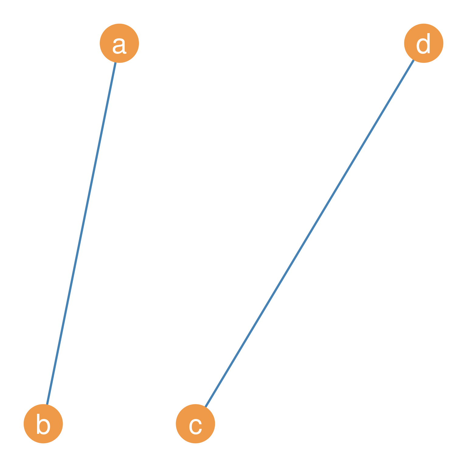
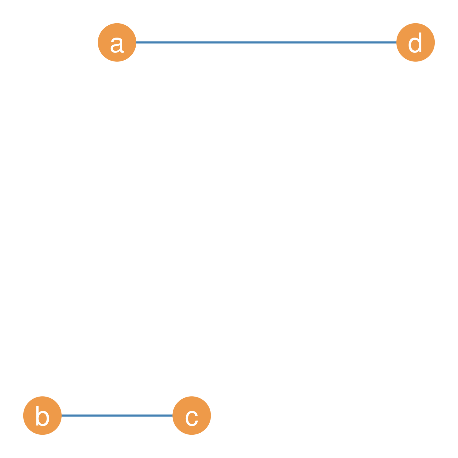
So, in the Figure fig-simple-1 case, the cardinality of the edge set is two \(|E| = 2\), and the cardinality of the vertex set is four \(|V| = 4\). These two basic graph properties are so important that they can serve as a “signature” for the graph. Sometimes people will refer to a graph as \(G(n, m)\) where \(n\) is the cardinality of the vertex set (number of nodes) and \(m\) is the cardinality of the edge set (number of edges). Thus, the graph in Figure fig-simple-1 is a \(G(4, 2)\) graph. Note that in Figure fig-simple-1, this is not the only possible \(G(4, 2)\) graph. Figure fig-simple-2 and Figure fig-simple-3 show two other possible variations of a \(G(4, 2)\) graph.
6.3 Graph Labeling
In Figure fig-simple-1, Figure fig-simple-2, and Figure fig-simple-3, the nodes have letters which function as “names” for each. Thus, we can refer to node \(A\), or node \(B\), and so forth. These names are arbitrary; we can also use numbers \(\{1, 2, 3, ...\}\) or a combination of letters and numbers \(\{V_1, V_2, V_3,... \}\).
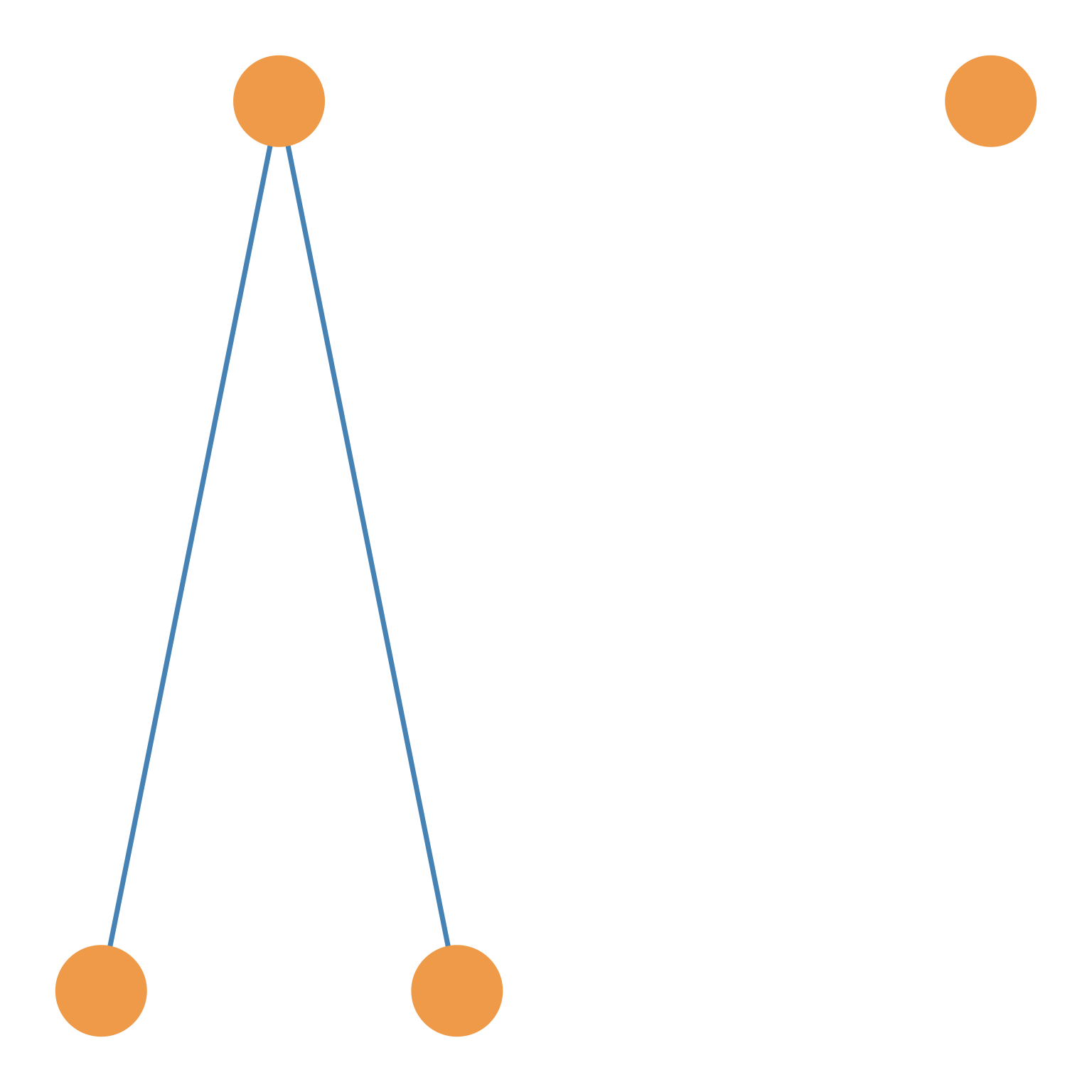
When the nodes of a graph are distinguished from one another using names, the graph is said to be labeled. Sometimes, the names don’t matter, so we don’t specify them, as in Figure fig-simple-4. In this case, the graph is said to be unlabeled.
Graph metrics, such as those we will compute starting at sec-graphmetrics, are the same regardless of whether the graph is labeled. Most of the example graphs we will look at are labeled.
6.4 Trivial and Non-Trivial Graphs
The \(G(1, 0)\) graph, essentially that formed by an isolated person sitting alone in a room with no connections to others (which can represent the case of the Japanese Hikikomori), is sometimes called the trivial graph. Obviously, for purposes of social network analysis, the graphs that are used are non-trivial.
The smallest non-trivial graph, and thus the smallest unit of social analysis, is the \(G(2, 1)\) graph, the social unit formed by two people connected by a single link, sometimes referred to as a connected dyad. Connected dyads are the “hydrogen atom” of society, the building block from which all other larger networks are built because all graphs can be thought of as larger lego block structures built by joining together various \(G(2, 1)\) graphs. The \(G(2, 0)\) graph, on the other hand, is a disconnected dyad, like two people stuck in a deserted island who decided to no longer speak to one another.
6.5 Basic Graph Properties
Graphs have some basic properties that we need to learn about:
- In a graph, if two nodes are joined together by an edge, they are said to be adjacent. So in Figure fig-simple-1, nodes A and B are adjacent, as are nodes A and C. Pairs of nodes that are not linked by an edge, like nodes B and C, are said to be nonadjacent.
- The nodes at the two ends of each existing edge are said to be the end vertices of that edge. Each edge has two end vertices. As we have been doing, edges are named by typing together the names of their two end vertices. So the edge with nodes A and B as endpoints is called AB.
- If an edge “touches” a node (e.g., connects it to another node), we say that that edge is incident on that node. So in Figure fig-simple-1, the edge AB is incident on both nodes A and B. The relation of incidence will be important in a later lesson when we discuss node-level network metrics, such as degree centrality.
- In a graph, nodes that are not connected to any other nodes are called isolates. This means that in Figure fig-simple-1, node D is an isolate because it has zero edges incident upon it.
- If a node is connected to \(n-1\) nodes in a graph—basically, every other node but themselves—it is called a star node or a dominant node. The star node is the opposite of an isolate, having the maximum number of connections that can be observed for a single node in a social network.
6.6 The Graph Complement
Sometimes, when examining a graph, we may be interested in its evil twin. This is called the graph complement.
More technically, for any graph \(G\), its complement \(G'\) is a graph that meets the following two conditions:
- Every pair of nodes adjacent in \(G\) is non-adjacent in \(G'\).
- Every pair of nodes that are non-adjacent in \(G\) and are adjacent in \(G'\).
That is, the disconnected nodes in graph \(G\) are connected in its complement \(G'\), and the connected nodes in \(G\) are disconnected in \(G'\).
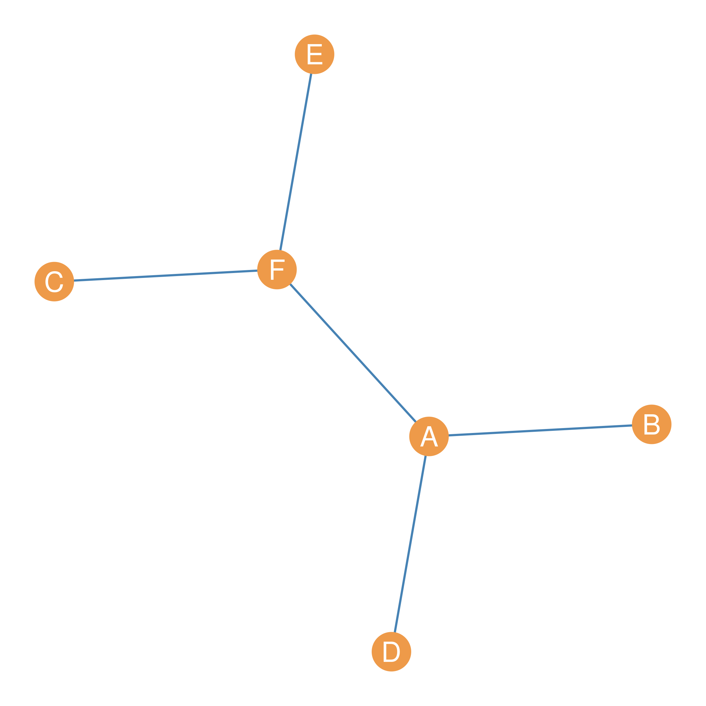
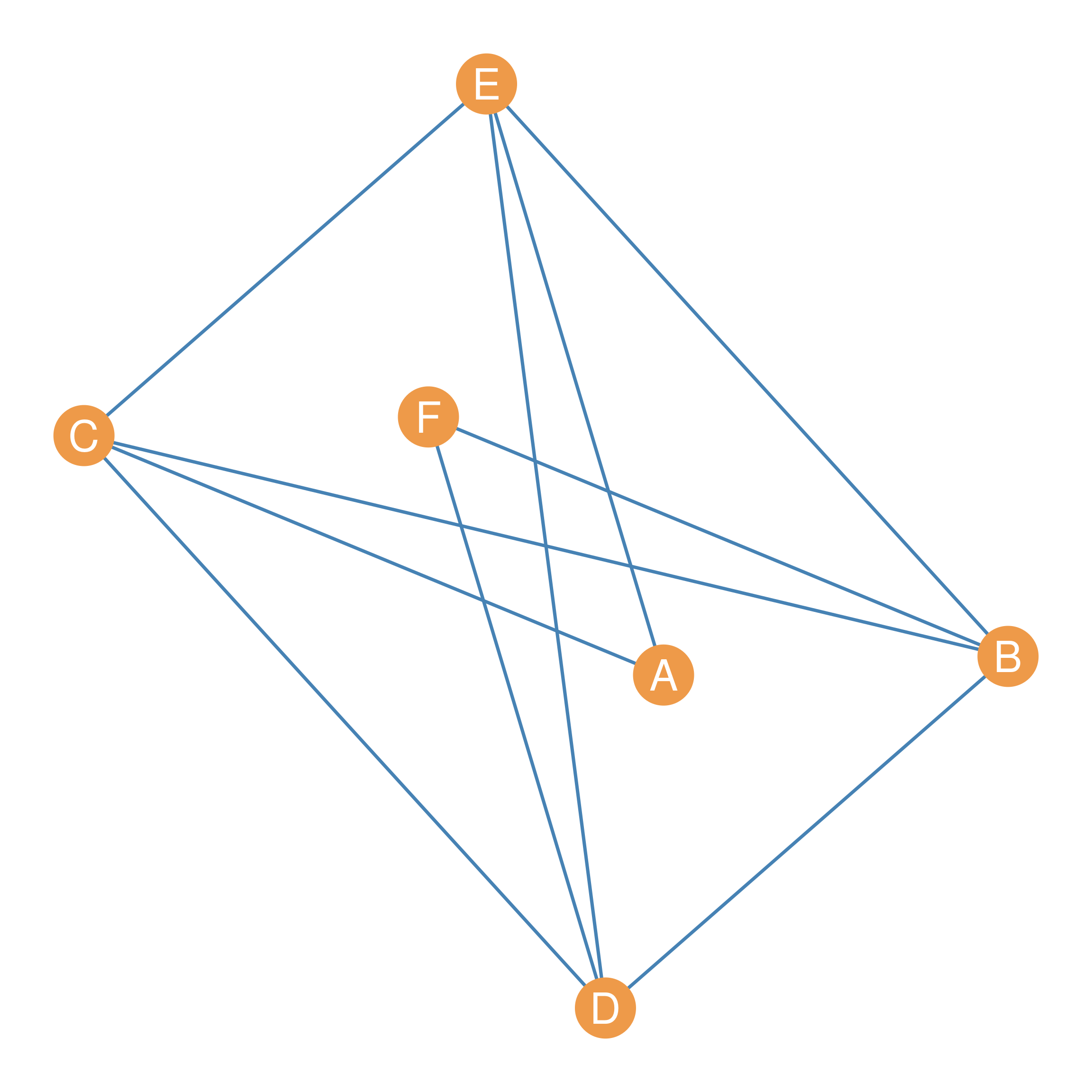
For instance, the \(G(6, 5)\) graph is shown in Figure fig-complement-1, namely a graph with six nodes and five edges, and the complement of that graph is shown in Figure fig-complement-2. As we can see, every pair of nodes that is connected in Figure fig-complement-1 is disconnected in Figure fig-complement-2 and vice versa.
What’s the graph complement useful for? As we will see later, we will sometimes be interested in counting the non-relations in a network, in addition to the relations. The complement (and its matrix representation) is useful for that.
6.7 Simple Graphs
Graphs like that shown in Figure fig-simple are called simple graphs. There are two requirements for a graph to count as a simple graph:
- First, there can only be one edge joining two nodes at any time. That is, there cannot be multiple lines linking together the same pair of nodes. We will see in a later lesson that certain types of graphs relax this restriction.
- The second requirement is that the graph does not contain any edges that have the same node as its two endpoints. These kinds of edges are called loops, and they are edges that connect a node to itself! Clearly, this does not make sense for most sociological applications.
With some exceptions, noted in subsequent lessons, simple graphs can represent most social networks.
6.8 Graphs are Not Pictures!
It is important to keep the mathematical notion of a “graph” (which is just a set of two sets of objects) from the idea of a “graph” that implies a visual representation or picture. The reason is that there is no true “picture” that represents a graph. The same mathematical graph can be represented in myriad of ways because the way we place the points and line in two dimensional space is completely arbitrary.
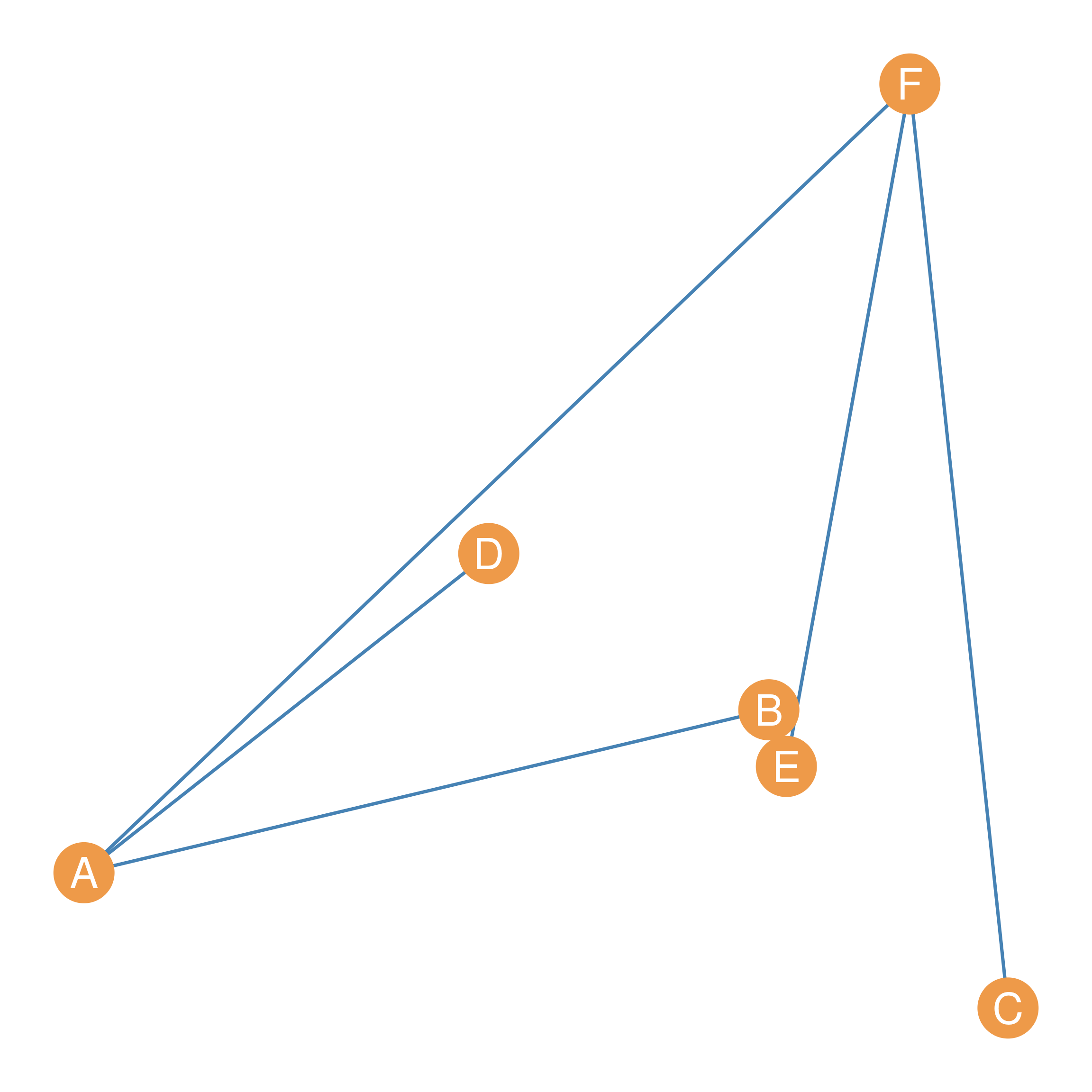
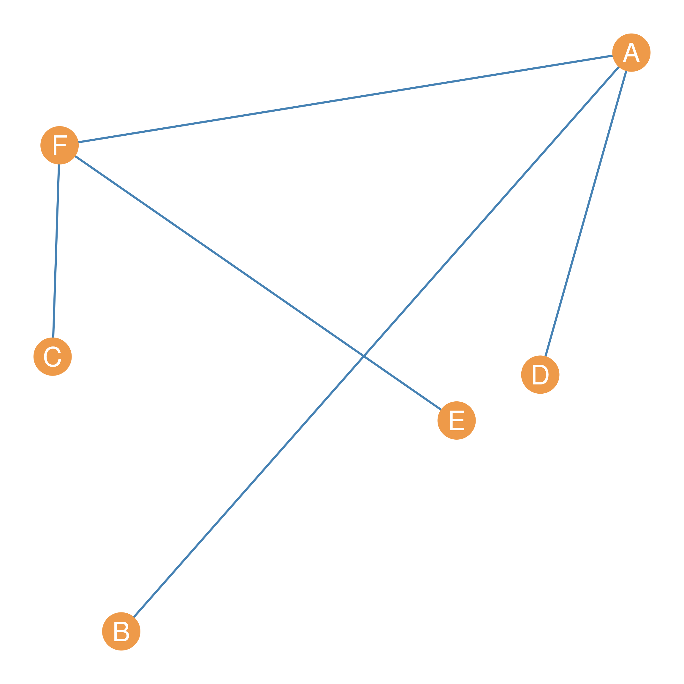
For instance, Figure fig-random-1 shows the same graph shown in Figure fig-complement-1, but with the points and lines positioned in a different way. Figure fig-random-1 and Figure fig-complement-1 are the same graph (they have the same set of nodes and the same set of edges) but as pictures, Figure fig-complement-1 and Figure fig-random-1 are pretty different. Note that Figure fig-random-2 is yet another way to draw the same graph, with the points and lines distributed differently in two-dimensional space.
6.9 Graphs and their Subgraphs
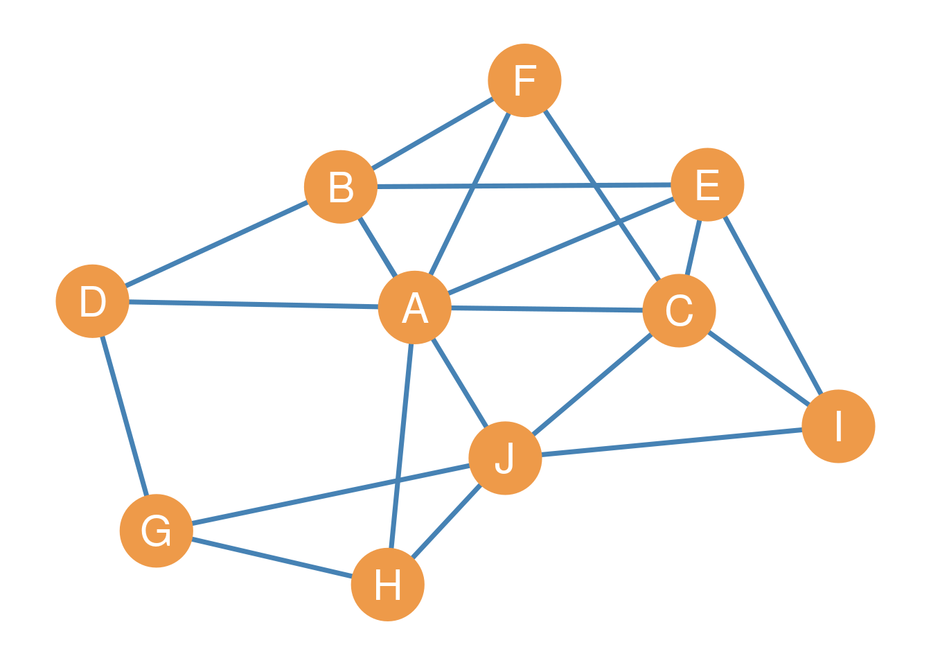
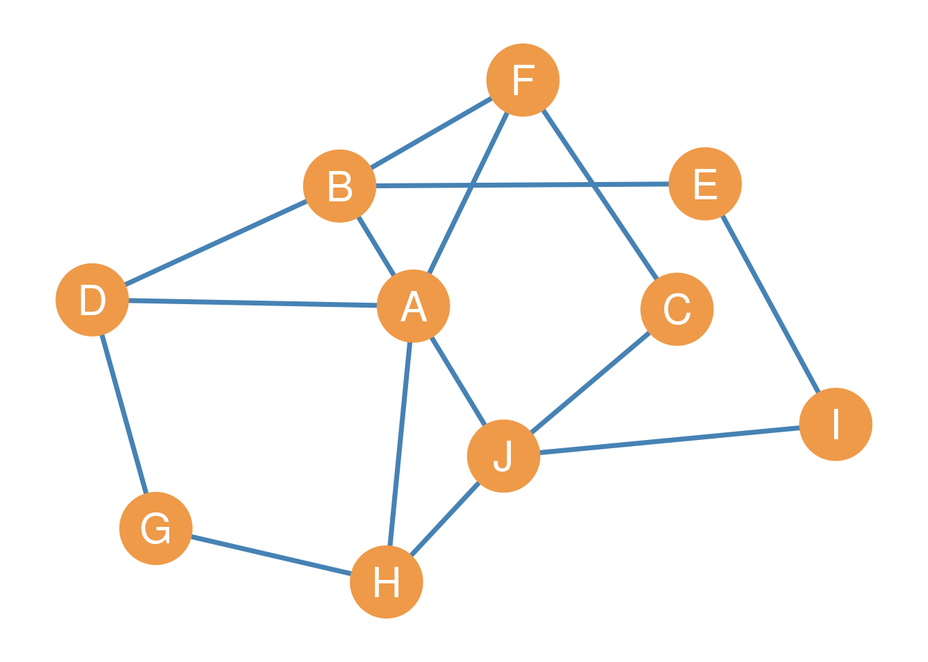
Consider the graph shown in Figure fig-subgraph-1. If all the actors that you are interested in studying are included here, we would refer to it as the whole network. However, sometimes, even when we collect data on a large number of actors, we may be interested in analyzing not the whole network, but only some parts of it. How do we do that?
Well, good thing a graph is actually a pair of sets. If you remember your high school set theory, you can always take a set and consider only a subset of the original members.
Since graphs are sets, we can do the same thing. A subset of the original nodes (or edges) of a graph is called a subgraph. So if \(G =\{E,V\}\) is the original graph, the subgraph \(G' = \{E',V'\}\) is a subset of \(G\), which is written \(G' \subset G\), with the understanding that \(E' \subset E\) and \(V' \subset V\). In mathematics, “\(\subset\)” is the symbol for subset. Thus, \(A \subset B\) is read as “set A is a subset of set B.”
For instance, let us say we are interested in just analyzing actors A, B, C, D, and E in the graph shown in Figure fig-subgraph-1. They seem to be a close-knit group. In that case, as noted earlier, if we call the original graph \(G\) with vertex and edge sets \(\{E, V\}\) we can define a new subgraph \(G'\), whose node subset \(V'\) only includes the actors we are interested in studying, in this case \(V' = \{A, B, C, D, E\}\), where \(V' \subset V\).
The subgraph \(G'\) is shown in Figure fig-subgraph-2. It looks exactly like we wanted, capturing the relations between an interconnected subgroup of actors in the original graph. Note that the edge set of the subgraph \(E'\) only includes those edges that are incident to the other nodes in the subgraph (as defined in sec-graphtheory) and omits those in the original graph that are incident to nodes that are not in the subgraph, so \(E' \subset E\). As we will see in a later lesson, well-connected subgroups of actors in an original graph are called cohesive subsets.
6.10 Vertex and Edge-Induced Subgraphs
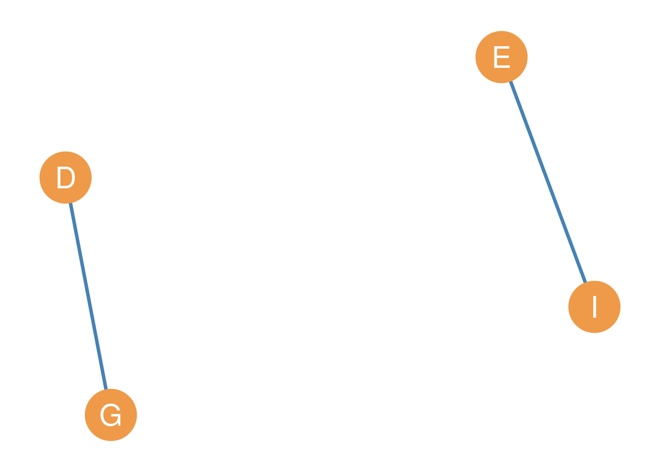
For any graph, we can define a subgraph based on any old random subset of the original node set. It is completely up to us. For instance, we could define a new subgraph \(G''\) of the original graph shown in Figure fig-subgraph-1, that includes the node set \(V'' = \{D, E, G, I\}\). That is shown in Figure fig-subgraph-3. That subgraph is weird (composed of two standalone connected dyads) and probably not very useful, but it is a subgraph of the original graph anyways!
Just like we can define subgraphs based on the node set of a graph, we can define subgraphs based on subsets of the original edge set. For instance, we could pick the edges \(E' = \{AB, AC, BJ\}\) and define a subgraph based on them, as shown in Figure fig-subgraph-edge-induced. This necessarily includes the node set \(V' = \{A, B, C, J\}\).
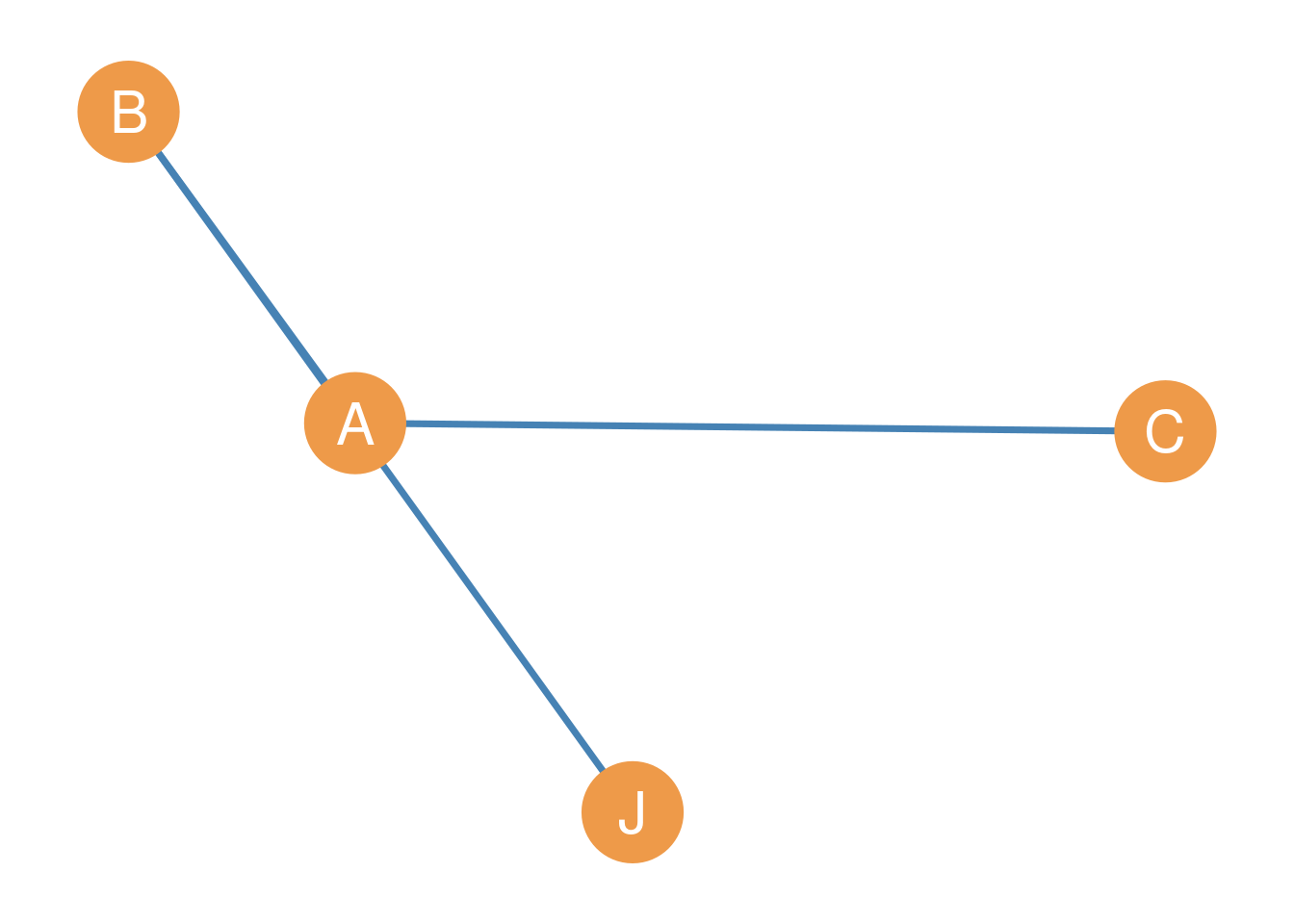
When a subgraph is defined by selecting a subset of nodes to retain (the common case), it is called a vertex-induced subgraph of the original graph, as in Figure fig-subgraph-2. When a subgraph is defined by picking a subset of edges from the original graph to keep, it is called (you guessed it) an edge-induced subgraph of the original graph.
6.11 Creating Subgraphs by Deleting Nodes and Edges
Another way to think about creating subgraphs is by deleting elements from the original graph. This approach is common in social network analysis when we want to see what a network would look like if certain actors or relationships were removed, which can help reveal how important they are for holding the network together.
6.11.1 Vertex-Deleted Subgraphs
It is possible to define a subgraph by deleting nodes. This is written as \(G' = G - \{a, b, c\}\), where \(\{a, b, c\}\) is the set of nodes being deleted. When you delete nodes, a critical rule applies: all edges incident to those nodes are automatically removed as well.
For example, starting with the graph in Figure fig-subgraph-1, if we delete the node set \(\{F, G, H, I, J\}\), the resulting subgraph is identical to the one shown in Figure fig-subgraph-2. This shows that a vertex-deleted subgraph can be equivalent to a vertex-induced subgraph. The action of deleting \(\{F, G, H, I, J\}\) induces a subgraph on the remaining nodes \(\{A, B, C, D, E\}\).
Two special cases of vertex deletion are: - The null graph, which results from removing all nodes from the original graph. - The singleton graph (or trivial graph), which results from removing all nodes except for one.
6.11.2 Edge-Deleted Subgraphs
Just as we can delete nodes, we can also create subgraphs by removing edges. This is written as \(G' = G - \{e_1, e_2, ...\}\), where \(\{e_1, e_2, ...\}\) is the set of edges being deleted. For instance, the edge-deleted subgraph in Figure fig-subgraph-4 results from removing the six edges \(\{AB, AE, AC, CI, CE, GJ\}\) from the graph in Figure fig-subgraph-1.
When you delete edges, the nodes that were connected by those edges remain in the graph. A subgraph created by removing only edges while leaving all original nodes intact is called a spanning subgraph.
A special case of edge deletion is the empty graph, which results from removing all edges from the original graph, leaving only the set of isolated nodes.
As we will see later, subgraphs (as well as vertex and edge deletion) are a useful concept for discussing levels at an “in-between” level, above the node level but “below” the whole network level: subgroups. However, subgraphs are also useful for network concepts at the node level, because there is a special type of subgraph, called the ego graph that is defined by picking a central node and the nodes that are connected to it, along with the edges connecting the nodes surrounding ego.
6.12 Nodes and their Neighborhoods
6.12.1 Node Neighborhoods
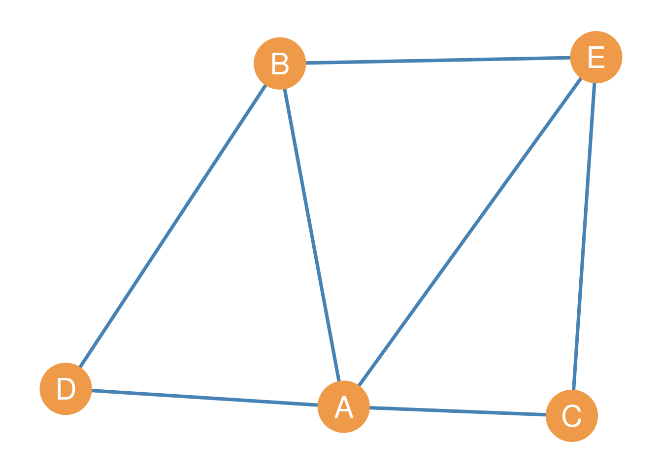
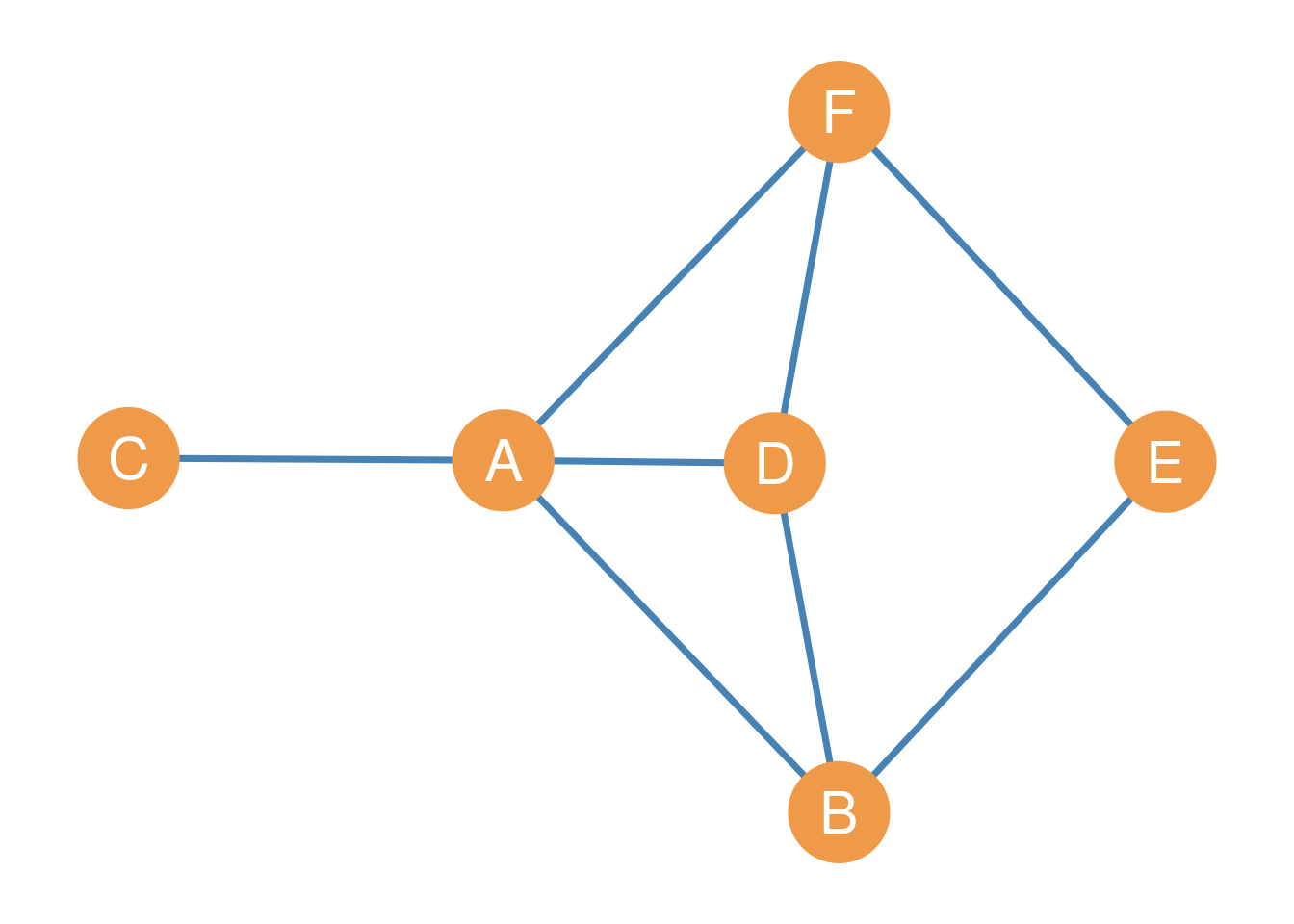
As we have seen, each node in a graph or order \(N\), given by the set \(V = \{v_1, v_2, v_3, \dots v_N\}\) may be adjacent to a certain set of other nodes. In graph theory, these are called the node’s neighbors. The neighborhood of a node in a graph is written as \(\mathcal{N}(v)\), where \(v\) is the node’s name in the graph. For instance, if we are referring to the neighbors of node A in the graph shown as Figure fig-simple2 we would write \(\mathcal{N}(A)\).
The neighborhood of each node is a proper subset of the larger set of nodes in the graph \(V\). This is written as \(\forall v: \mathcal{N}(v) \subset V\), which translates from math to English as “for all nodes \(v\), the neighborhood of \(v\) is a subset of the larger node set \(V\).” In Figure fig-simple2 for instance, \(\mathcal{N}(A) = \{B, C, D, F\}\), and \(\mathcal{N}(A) \subset V\).1
1 The mathematical symbol for subset is \(\subset\).
6.12.1.1 Node Neighborhood Intersection
Note that the neighbor sets of two nodes can have members in common. For instance, in Figure fig-simple2 we have \(\mathcal{N}(A) = \{B, C, D, F\}\) and we also have \(\mathcal{N}(D) = \{A, B, F\}\). These two sets share common members!
Sometimes, we may be interested in the total number of other people that two nodes share a connection with. Like when you wonder how many people you and your friend are both friends with (or a social media algorithm lets you know). This is called the intersection of the two node neighborhood sets.
So if A and D are both nodes in a graph, the intersection of their neighborhood sets gives us a list of the other nodes in the graph they are both connected to. Using set theory notation, this can be written as: \(\mathcal{N}(A) \cap \mathcal{N}(D) = \{B, F\}\), which says that nodes A and D have B and F as common neighbors.2
2 The mathematical symbol for set intersection is \(\cap\).
The cardinality of the sets formed by the intersection of the neighborhoods of all the nodes in the graph gives us the number of common neighbors between each pair of nodes, which may be zero if two neighborhood sets are disjoint. As we saw in sec-graphtheory, in set theory, the cardinality of a set is the number of its members. Thus, the cardinality of the set \(\{A, B, C, D\}\) is four. Two sets are disjoint if they have no members in common, meaning their intersection is the empty set. We will see in a later lesson that this quantity has applications for deriving important matrices from graphs and for computing key network metrics.
Note that two nodes can have common neighbors even if they are not directly connected in the network! So the number of common neighbors is defined for both connected and null dyads.
For instance, in Figure fig-simple2, the intersection of the neighborhoods of nodes D and E exists and it is given by \(\mathcal{N}(D) \cap \mathcal{N}(E) = \{B, F\}\) even though nodes D and E are not linked (they are nonadjacent).
6.12.1.2 Node Neighborhood Union
Sometimes we may be interested in the total number of other people that two nodes are connected to, regardless of whether both of them are connected to them. Think of this as adding the set of people that you know with the set of people one of your friends knows, counting the people that your friend knows but you don’t, and the people you know but your friend doesn’t. This is called the union of the two node neighborhood sets.
So if A and D are both nodes in a graph, the union of their neighborhood sets gives us a list of the total number of other nodes in the graph either one is connected to.
Using set theory notation, this can be written as:3
3 The mathematical symbol for set union is \(\cup\).
\[ \mathcal{N}(A) \cup \mathcal{N}(D) = \{B, C, F\} \tag{6.5}\]
Which states that nodes A and D have B and C as neighbors, but not necessarily common neighbors.
As we will see later, the intersection and union of neighborhood sets can serve as a basis for constructing measures of (structural) similarity between nodes in a graph.
6.12.2 Node Degree
In an undirected graph, a given node’s degree can be defined in two ways, both of which lead to the same answer.
One way to think about the degree of a given node \(i\) in a graph (written \(k_i\)) is as the cardinality of the set of neighbors of that node as defined earlier:
\[ k_i = |\mathcal{N}(i)| \tag{6.6}\]
So in the graph shown in Figure fig-simple2:
\[ k_A = |\mathcal{N}(A)| = |\{B, C, D, F\}|=4 \tag{6.7}\]
Another way to think about node degree is not as the cardinality of the node neighborhood set, but as a count of edges. In this case, we count the number of edges that have a given node \(i\) as one of their endpoints. Recall that an edge that has a given node as one of its endpoints is said to be incident upon that node. So in the graph shown in Figure fig-simple2, the set of edges that have node A as one of their endpoints is:
\[ k_A = \{AB, AC, AD, AF\} \]
Which means that:
\[ |k_A| = 4 \] Either way, computing the degree of a node as the cardinality of its neighbor set or as the number of edges incident upon the node gives us the number of other people a given node is connected to in the network. We will see when we talk about centrality, that this is an important measure of node position called degree centrality (Freeman 1977).
Freeman, Linton C. 1977. “A Set of Measures of Centrality Based on Betweenness.” Sociometry 40 (1): 35–41.
In a graph, nodes that have a degree equal to one, and thus have just a single neighbor in the graph, are called endpoints of the graph. Thus, in Figure fig-simple2, node \(C\) is an endpoint.