| 50 | 72 | 46 | 47 | 46 |
| 72 | 139 | 88 | 74 | 71 |
| 46 | 88 | 56 | 46 | 46 |
| 47 | 74 | 46 | 50 | 41 |
| 46 | 71 | 46 | 41 | 45 |
17 Matrix Multiplication and its Applications
Matrix multiplication (symbol: \(\times\) or \(\cdot\) or %*% in R) is perhaps the most mathematically complex of the basic matrix algebra operations we will cover. While its mechanics are slightly involved, its applications in social network analysis are profound. It allows us to calculate indirect connections (walks), identify cohesive subgroups (cliques), and find the number of common neighbors shared by pairs of nodes.
We will begin by laying out the mathematical rules of matrix multiplication before exploring its extensive applications in network science.
17.1 Matrix Multiplication Rules
First, we must understand the conditions under which two matrices can be multiplied:
- Conformability: You can always multiply two matrices as long as the number of columns of the first matrix equals the number of rows of the second matrix. To check this, line up their dimensions side-by-side:
\[ \mathbf{A}_{3 \times \mathbf{5}} \times \mathbf{B}_{\mathbf{5} \times 6} \]
- Inner Dimensions: The two “fives” in bold are called the inner dimensions. The “three” on the left and the “six” on the right are called the outer dimensions. Matrix multiplication is defined only if their inner dimensions are equal. When they match, the matrices are conformable; otherwise, they are non-conformable and cannot be multiplied.
- Order Matters: Unlike numbers, where the order of multiplication does not matter (\(4 \times 3 = 3 \times 4\)), matrix multiplication is non-commutative. For almost all matrices \(\mathbf{A}\) and \(\mathbf{B}\):
\[ \mathbf{A} \times \mathbf{B} \neq \mathbf{B} \times \mathbf{A} \]
- Resulting Dimensions: The resulting product matrix will always have dimensions equal to the outer dimensions of the two multipliers:
\[ \mathbf{A}_{3 \times \mathbf{5}} \times \mathbf{B}_{\mathbf{5} \times 6} = \mathbf{C}_{3 \times 6} \tag{17.1}\]
17.2 Multiplying a Matrix Times its Transpose
By definition, the rows of a matrix are equal to the columns of its transpose, and vice-versa. Therefore, the product of a matrix times its transpose, and the transpose times the original matrix, is always defined, regardless of the original matrix’s dimensions. Thus:
\[ \mathbf{A} \times \mathbf{A}^T = \text{Always Defined!} \]
\[ \mathbf{A}^T \times \mathbf{A} = \text{Always Defined!} \]
When you multiply a matrix of dimensions \(m \times n\) by its transpose (\(n \times m\)), the resulting matrix will always be a square matrix of dimensions \(m \times m\):
\[ \mathbf{A}_{5 \times 3} \times \mathbf{A}_{3 \times 5}^T = \mathbf{B}_{5 \times 5} \tag{17.2}\]
Conversely, reversing the order yields a square matrix of dimensions \(n \times n\):
\[ \mathbf{A}_{3 \times 5}^T \times \mathbf{A}_{5 \times 3} = \mathbf{B}_{3 \times 3} \tag{17.3}\]
17.3 Matrix Powers
You can multiply a matrix times itself to calculate matrix powers (\(A^n\)), but only if the matrix is a square matrix (having the same number of rows and columns). Thus:
\[ \mathbf{A}^2 = \mathbf{A} \times \mathbf{A} \]
\[ \mathbf{A}^3 = \mathbf{A} \times \mathbf{A} \times \mathbf{A} \]
\[ \mathbf{A}^n = \mathbf{A} \times \mathbf{A} \times \dots \times \mathbf{A} \]
Since the adjacency matrices used to represent social networks are always square matrices, we can always find the powers of an adjacency matrix.
When you multiply a square matrix by another square matrix of the same dimensions, the resulting matrix is always of the same dimensions:
\[ \mathbf{A}_{5 \times 5} \times \mathbf{A}_{5 \times 5} = \mathbf{A}^2_{5 \times 5} \]
17.4 Numerical Multiplication Examples
Let’s see some numeric examples of how matrix multiplication works. Table tbl-trans displays an original matrix \(\mathbf{A}\) and its transpose \(\mathbf{A}^T\).
| 3 | 4 | 5 |
| 7 | 9 | 3 |
| 4 | 6 | 2 |
| 5 | 3 | 4 |
| 2 | 5 | 4 |
| 3 | 7 | 4 | 5 | 2 |
| 4 | 9 | 6 | 3 | 5 |
| 5 | 3 | 2 | 4 | 4 |
Table tbl-prod shows the result of multiplying the \(5 \times 3\) matrix \(\mathbf{A}\) times its \(3 \times 5\) transpose \(\mathbf{A}^T\):
Where do these numbers come from? Let’s trace a couple of cells: 1. Cell (Row 1, Column 1) = 50: We multiply the elements of the first row of \(\mathbf{A}\) (\(\{3, 4, 5\}\)) by the corresponding elements of the first column of \(\mathbf{A}^T\) (\(\{3, 4, 5\}\)), and sum them up:
\[ (3 \times 3) + (4 \times 4) + (5 \times 5) = 9 + 16 + 25 = 50 \]
Cell (Row 4, Column 2) = 74: We multiply the elements of the fourth row of \(\mathbf{A}\) (\(\{5, 3, 4\}\)) by the corresponding elements of the second column of \(\mathbf{A}^T\) (\(\{7, 9, 3\}\)), and sum them:
\[ (5 \times 7) + (3 \times 9) + (4 \times 3) = 35 + 27 + 12 = 74 \]
We repeat this process for all 25 cells to obtain the complete product matrix. Note that the resulting product matrix \(\mathbf{B}\) is symmetric (\(b_{ij} = b_{ji}\)).
Reversing the order and multiplying \(\mathbf{A}^T \times \mathbf{A}\) yields a smaller \(3 \times 3\) square matrix, as shown in Table tbl-prod2:
| 103 | 124 | 72 |
| 124 | 167 | 91 |
| 72 | 91 | 70 |
To find the cell at (Row 3, Column 1) = 72, we multiply the third row of \(\mathbf{A}^T\) (\(\{5, 3, 2, 4, 4\}\)) by the first column of \(\mathbf{A}\) (\(\{3, 7, 4, 5, 2\}\)):
\[ (5 \times 3) + (3 \times 7) + (2 \times 4) + (4 \times 5) + (4 \times 2) = 15 + 21 + 8 + 20 + 8 = 72 \]
17.5 Matrix Powers and Indirect Connections in Social Networks
Taking the powers of an adjacency matrix was one of the earliest applications of formal social network analysis, co-discovered by Duncan Luce and Albert Perry (1949) and Leon Festinger (1949).
Luce, RD, and Albert D Perry. 1949. “A Method of Matrix Analysis of Group Structure.” Psychometrika 14 (2): 95–116.
Festinger, Leon. 1949. “The Analysis of Sociograms Using Matrix Algebra.” Human Relations 2 (2): 153–58.
When we calculate the powers of an adjacency matrix, the resulting entries have an intuitive and powerful interpretation: they count the exact number of indirect connections (walks) of a given length between each pair of people.
Let’s explore this using the 12-person “hanging out” network shown in Figure fig-rel-1. Table tbl-pows shows the original binary adjacency matrix \(\mathbf{A}\), its square \(\mathbf{A}^2\), and its cube \(\mathbf{A}^3\).
| A | B | C | D | E | F | G | H | I | J | K | L | |
|---|---|---|---|---|---|---|---|---|---|---|---|---|
| A | 0 | 0 | 1 | 1 | 0 | 0 | 0 | 0 | 0 | 0 | 0 | 0 |
| B | 0 | 0 | 1 | 1 | 0 | 0 | 0 | 0 | 0 | 0 | 0 | 0 |
| C | 1 | 1 | 0 | 1 | 0 | 0 | 0 | 1 | 0 | 0 | 0 | 0 |
| D | 1 | 1 | 1 | 0 | 0 | 0 | 0 | 0 | 0 | 0 | 0 | 1 |
| E | 0 | 0 | 0 | 0 | 0 | 1 | 1 | 1 | 0 | 1 | 0 | 0 |
| F | 0 | 0 | 0 | 0 | 1 | 0 | 1 | 1 | 0 | 0 | 0 | 0 |
| G | 0 | 0 | 0 | 0 | 1 | 1 | 0 | 1 | 0 | 0 | 0 | 0 |
| H | 0 | 0 | 1 | 0 | 1 | 1 | 1 | 0 | 0 | 0 | 0 | 0 |
| I | 0 | 0 | 0 | 0 | 0 | 0 | 0 | 0 | 0 | 1 | 1 | 1 |
| J | 0 | 0 | 0 | 0 | 1 | 0 | 0 | 0 | 1 | 0 | 0 | 1 |
| K | 0 | 0 | 0 | 0 | 0 | 0 | 0 | 0 | 1 | 0 | 0 | 0 |
| L | 0 | 0 | 0 | 1 | 0 | 0 | 0 | 0 | 1 | 1 | 0 | 0 |
| A | B | C | D | E | F | G | H | I | J | K | L | |
|---|---|---|---|---|---|---|---|---|---|---|---|---|
| A | 2 | 2 | 1 | 1 | 0 | 0 | 0 | 1 | 0 | 0 | 0 | 1 |
| B | 2 | 2 | 1 | 1 | 0 | 0 | 0 | 1 | 0 | 0 | 0 | 1 |
| C | 1 | 1 | 4 | 2 | 1 | 1 | 1 | 0 | 0 | 0 | 0 | 1 |
| D | 1 | 1 | 2 | 4 | 0 | 0 | 0 | 1 | 1 | 1 | 0 | 0 |
| E | 0 | 0 | 1 | 0 | 4 | 2 | 2 | 2 | 1 | 0 | 0 | 1 |
| F | 0 | 0 | 1 | 0 | 2 | 3 | 2 | 2 | 0 | 1 | 0 | 0 |
| G | 0 | 0 | 1 | 0 | 2 | 2 | 3 | 2 | 0 | 1 | 0 | 0 |
| H | 1 | 1 | 0 | 1 | 2 | 2 | 2 | 4 | 0 | 1 | 0 | 0 |
| I | 0 | 0 | 0 | 1 | 1 | 0 | 0 | 0 | 3 | 1 | 0 | 1 |
| J | 0 | 0 | 0 | 1 | 0 | 1 | 1 | 1 | 1 | 3 | 1 | 1 |
| K | 0 | 0 | 0 | 0 | 0 | 0 | 0 | 0 | 0 | 1 | 1 | 1 |
| L | 1 | 1 | 1 | 0 | 1 | 0 | 0 | 0 | 1 | 1 | 1 | 3 |
| A | B | C | D | E | F | G | H | I | J | K | L | |
|---|---|---|---|---|---|---|---|---|---|---|---|---|
| A | 2 | 2 | 6 | 6 | 1 | 1 | 1 | 1 | 1 | 1 | 0 | 1 |
| B | 2 | 2 | 6 | 6 | 1 | 1 | 1 | 1 | 1 | 1 | 0 | 1 |
| C | 6 | 6 | 4 | 7 | 2 | 2 | 2 | 7 | 1 | 2 | 0 | 2 |
| D | 6 | 6 | 7 | 4 | 2 | 1 | 1 | 2 | 1 | 1 | 1 | 6 |
| E | 1 | 1 | 2 | 2 | 6 | 8 | 8 | 9 | 1 | 6 | 1 | 1 |
| F | 1 | 1 | 2 | 1 | 8 | 6 | 7 | 8 | 1 | 2 | 0 | 1 |
| G | 1 | 1 | 2 | 1 | 8 | 7 | 6 | 8 | 1 | 2 | 0 | 1 |
| H | 1 | 1 | 7 | 2 | 9 | 8 | 8 | 6 | 1 | 2 | 0 | 2 |
| I | 1 | 1 | 1 | 1 | 1 | 1 | 1 | 1 | 2 | 5 | 3 | 5 |
| J | 1 | 1 | 2 | 1 | 6 | 2 | 2 | 2 | 5 | 2 | 1 | 5 |
| K | 0 | 0 | 0 | 1 | 1 | 0 | 0 | 0 | 3 | 1 | 0 | 1 |
| L | 1 | 1 | 2 | 6 | 1 | 1 | 1 | 2 | 5 | 5 | 1 | 2 |
17.5.1 The Squared Adjacency Matrix (\(\mathbf{A}^2\))
What do the entries in Table tbl-pows-2 mean?
- Off-Diagonal Entries: The value in cell \(a^2_{ij}\) tells us the exact number of walks of length 2 between node \(i\) and node \(j\) (see sec-indirect). For example, \(a^2_{AB} = 2\). Looking at Figure fig-rel-1, we see that \(A\) can reach \(B\) via exactly two walks of length 2: \(\{AC, CB\}\) and \(\{AD, DB\}\). Similarly, \(a^2_{AC} = 1\), representing the walk \(\{AD, DC\}\).
- Diagonal Entries: The diagonal entry \(a^2_{ii}\) counts the number of walks of length 2 that begin and end with node \(i\). Since a walk of length 2 that goes from \(i \to j \to i\) in an undirected graph simply represents traversing an edge and returning, the diagonal of \(\mathbf{A}^2\) is equal to the degree of each node!
17.5.2 The Cubed Adjacency Matrix (\(\mathbf{A}^3\))
What do the entries in Table tbl-pows-3 mean?
- Off-Diagonal Entries: Tell us the exact number of walks of length 3 linking each pair of nodes. For instance, \(a^3_{HF} = 1\). Looking at the graph, this corresponds to the walk \(\{HG, GE, EF\}\).
- Diagonal Entries: Count the number of walks of length 3 that begin and end at the same node (which is a cycle of length 3). A cycle of length 3 is structurally equivalent to a clique of size 3 (a triangle)! The diagonal entry \(a^3_{ii}\) counts exactly twice the number of triangles node \(i\) belongs to (once going clockwise, and once counterclockwise). Thus, dividing the diagonal entries of \(\mathbf{A}^3\) by two tells us exactly how many triangles (cliques of size 3) each node belongs to. For instance, node \(K\) belongs to no triangles, so \(a^3_{KK} = 0\).
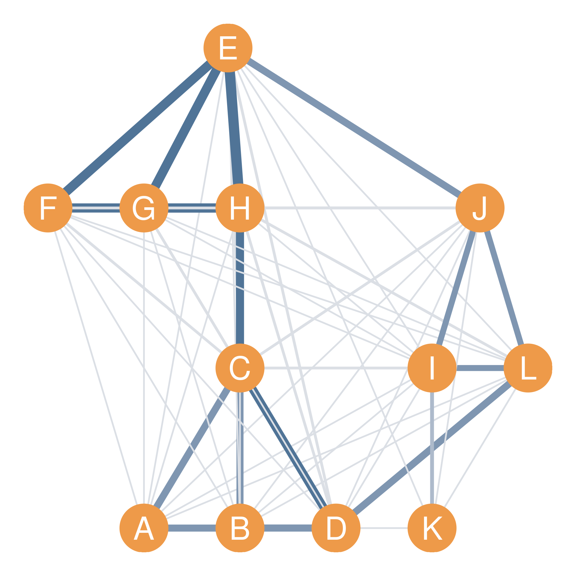
Figure fig-pows redraws our hangout network, but scales the edge widths and color intensity based on the entries in \(\mathbf{A}^3\). This immediately highlights cohesive cliques (like the subgroups \(\{A, B, C, D\}\) and \(\{E, F, G, H\}\)) which are densely bound together by extensive indirect connections.
17.6 Matrix Multiplication of Vectors
Recall that a vector is a sequence of numbers of a given length. A vector is actually just a special case of a matrix: * Row Vector: A matrix with one row and as many columns as the vector’s length (\(\mathbf{a}_{1 \times n}\)). * Column Vector: A matrix with one column and as many rows as the vector’s length (\(\mathbf{a}^T_{n \times 1}\)).
An example of a row vector \(\mathbf{a} = \{2, 4, 7, 2, 4\}\) of dimensions \(1 \times 5\) is shown in Table tbl-vecmat, and its \(5 \times 1\) transpose column vector \(\mathbf{a}^T\) is shown in Table tbl-transvec.
| 2 | 4 | 7 | 2 | 4 |
| 2 |
| 4 |
| 7 |
| 2 |
| 4 |
17.6.1 Vector Multiplication Rules
- Row Vector times Column Vector: Since this matches a matrix times its transpose, the product is always defined. The output is always a \(1 \times 1\) “matrix,” which is a single number (a scalar):
\[ \mathbf{a}_{1 \times 5} \times \mathbf{a}^T_{5 \times 1} = b_{1 \times 1} \tag{17.4}\]
\[ (2 \times 2) + (4 \times 4) + (7 \times 7) + (2 \times 2) + (4 \times 4) = 4 + 16 + 49 + 4 + 16 = 89 \]
- Column Vector times Row Vector: Reversing the order multiplies a \(5 \times 1\) column vector by a \(1 \times 5\) row vector, yielding a \(5 \times 5\) square matrix (shown in Table tbl-transvec2):
\[ \mathbf{a}^T_{5 \times 1} \times \mathbf{a}_{1 \times 5} = \mathbf{B}_{5 \times 5} \tag{17.5}\]
| 4 | 8 | 14 | 4 | 8 |
| 8 | 16 | 28 | 8 | 16 |
| 14 | 28 | 49 | 14 | 28 |
| 4 | 8 | 14 | 4 | 8 |
| 8 | 16 | 28 | 8 | 16 |
17.7 Multiplying a Vector Times a Matrix (and Vice Versa)
We can multiply a vector times a matrix (and a matrix times a vector) following the standard rules of conformability:
17.7.1 1. Row Vector Times Matrix
Multiplying a \(1 \times n\) row vector by an \(n \times m\) matrix yields another row vector of dimensions \(1 \times m\):
\[ \mathbf{b}_{1 \times 4} \times \mathbf{A}_{4 \times 4} = \mathbf{c}_{1 \times 4} \tag{17.6}\]
| 4 | 9 | 3 | 5 |
| 0 | 1 | 0 | 1 |
| 0 | 1 | 1 | 0 |
| 1 | 0 | 1 | 1 |
| 1 | 0 | 1 | 0 |
| 8 | 13 | 17 | 7 |
17.7.2 2. Matrix Times Column Vector
Multiplying an \(m \times n\) matrix by an \(n \times 1\) column vector yields another column vector of dimensions \(m \times 1\):
\[ \mathbf{A}_{5 \times 5} \times \mathbf{b}_{5 \times 1} = \mathbf{c}_{5 \times 1} \tag{17.7}\]
17.8 Matrix Times the “All Ones” Vector: Summing Row and Columns
In matrix algebra, the all ones vector (symbol: \(\mathbf{1}\)) is a special vector consisting entirely of ones. It has an incredibly useful property in social network analysis: it acts as a summation tool.
17.8.1 1. Row Vector of All Ones (\(\mathbf{1}_{1 \times n}\))
If you multiply the \(1 \times n\) row vector of all ones by any square adjacency matrix \(\mathbf{A}\), the product is a row vector containing the column sums of the matrix (equivalent to the indegrees of each node in a directed graph!):
\[ \mathbf{1}_{1 \times 5} \times \mathbf{A}_{5 \times 5} = \mathbf{b}_{1 \times 5} \tag{17.8}\]
| 1 | 1 | 1 | 1 | 1 |
| 0 | 1 | 0 | 1 | 0 |
| 1 | 1 | 0 | 1 | 0 |
| 1 | 1 | 1 | 0 | 1 |
| 0 | 1 | 1 | 0 | 0 |
| 1 | 1 | 0 | 1 | 0 |
| 3 | 5 | 2 | 3 | 1 |
17.8.2 2. Column Vector of All Ones (\(\mathbf{1}^T_{n \times 1}\))
If you multiply a square adjacency matrix \(\mathbf{A}\) by the \(n \times 1\) column vector of all ones, the product is a column vector containing the row sums of the matrix (equivalent to the outdegrees of each node!):
\[ \mathbf{A}_{5 \times 5} \times \mathbf{1}^T_{5 \times 1} = \mathbf{b}_{5 \times 1} \tag{17.9}\]
| 0 | 1 | 0 | 1 | 0 |
| 1 | 1 | 0 | 1 | 0 |
| 1 | 1 | 1 | 0 | 1 |
| 0 | 1 | 1 | 0 | 0 |
| 1 | 1 | 0 | 1 | 0 |
| 1 |
| 1 |
| 1 |
| 1 |
| 1 |
| 2 |
| 3 |
| 4 |
| 2 |
| 3 |
Thus, multiplying by the all-ones vector is the formal algebraic way to sum rows and columns!
17.9 The Identity Matrix
The identity matrix (symbol: \(\mathbf{I}\)) is a square matrix of dimensions \(n \times n\) with “1” in every diagonal cell, and “0” in every off-diagonal cell.
| 1 | 0 | 0 | 0 | 0 |
| 0 | 1 | 0 | 0 | 0 |
| 0 | 0 | 1 | 0 | 0 |
| 0 | 0 | 0 | 1 | 0 |
| 0 | 0 | 0 | 0 | 1 |
In matrix algebra, \(\mathbf{I}\) serves as the multiplicative identity (equivalent to the number “1” in regular arithmetic). Multiplying any conformable square matrix \(\mathbf{A}\) by the identity matrix yields the original matrix unchanged:
\[ \mathbf{A} \times \mathbf{I} = \mathbf{A} \tag{17.10}\]
\[ \mathbf{I} \times \mathbf{A} = \mathbf{A} \tag{17.11}\]
17.10 Matrix Multiplication and Common Neighbors
What happens when we multiply a network’s adjacency matrix (\(\mathbf{A}\)) by its transpose (\(\mathbf{A}^T\))?
\[ \mathbf{A} \times \mathbf{A}^T = \mathbf{B} \]
Let’s calculate this product for our running 12-person hangout network. The resulting matrix \(\mathbf{B}\) is shown in Table tbl-comm:
| A | B | C | D | E | F | G | H | I | J | K | L | |
|---|---|---|---|---|---|---|---|---|---|---|---|---|
| A | 2 | 2 | 1 | 1 | 0 | 0 | 0 | 1 | 0 | 0 | 0 | 1 |
| B | 2 | 2 | 1 | 1 | 0 | 0 | 0 | 1 | 0 | 0 | 0 | 1 |
| C | 1 | 1 | 4 | 2 | 1 | 1 | 1 | 0 | 0 | 0 | 0 | 1 |
| D | 1 | 1 | 2 | 4 | 0 | 0 | 0 | 1 | 1 | 1 | 0 | 0 |
| E | 0 | 0 | 1 | 0 | 4 | 2 | 2 | 2 | 1 | 0 | 0 | 1 |
| F | 0 | 0 | 1 | 0 | 2 | 3 | 2 | 2 | 0 | 1 | 0 | 0 |
| G | 0 | 0 | 1 | 0 | 2 | 2 | 3 | 2 | 0 | 1 | 0 | 0 |
| H | 1 | 1 | 0 | 1 | 2 | 2 | 2 | 4 | 0 | 1 | 0 | 0 |
| I | 0 | 0 | 0 | 1 | 1 | 0 | 0 | 0 | 3 | 1 | 0 | 1 |
| J | 0 | 0 | 0 | 1 | 0 | 1 | 1 | 1 | 1 | 3 | 1 | 1 |
| K | 0 | 0 | 0 | 0 | 0 | 0 | 0 | 0 | 0 | 1 | 1 | 1 |
| L | 1 | 1 | 1 | 0 | 1 | 0 | 0 | 0 | 1 | 1 | 1 | 3 |
This resulting matrix \(\mathbf{B}\) contains two incredibly valuable pieces of network information:
- Diagonal Entries (\(b_{ii}\)): The diagonal entries count the degree of each node. This is because multiplying row \(i\) by column \(i\) (which is identical in a symmetric matrix) squares each binary entry and sums them, giving the total number of neighbors node \(i\) has.
- Off-Diagonal Entries (\(b_{ij}\)): The off-diagonal entries count the exact number of common neighbors shared by node \(i\) and node \(j\)!
Let’s trace why this happens. Look at \(b_{AC} = 1\) (Row A, Column C). This entry is obtained by multiplying the first row of the adjacency matrix (representing \(A\)’s connections) by the third column of the adjacency matrix (representing \(C\)’s connections), as shown in Table tbl-commex:
| A | B | C | D | E | F | G | H | I | J | K | L |
|---|---|---|---|---|---|---|---|---|---|---|---|
| 0 | 0 | 1 | 1 | 0 | 0 | 0 | 0 | 0 | 0 | 0 | 0 |
| A | B | C | D | E | F | G | H | I | J | K | L |
|---|---|---|---|---|---|---|---|---|---|---|---|
| 1 | 1 | 0 | 1 | 0 | 0 | 0 | 1 | 0 | 0 | 0 | 0 |
| A | B | C | D | E | F | G | H | I | J | K | L |
|---|---|---|---|---|---|---|---|---|---|---|---|
| 0 | 0 | 0 | 1 | 0 | 0 | 0 | 0 | 0 | 0 | 0 | 0 |
The cell-by-cell product vector shown in Table tbl-commex-3 contains a “1” only in the position corresponding to node \(D\). Because both \(A\) and \(C\) are connected to \(D\), the product of their ties to \(D\) is \(1 \times 1 = 1\). For any node they do not both share as a neighbor, the product is 0.
Summing up this product vector yields \(1\), confirming that node \(D\) is the single, shared common neighbor between \(A\) and \(C\).
Thus, multiplying an adjacency matrix by its transpose is the formal algebraic way to map out all common neighbors in a network!
TipAssociated Assignment on Bruin Learn
Now that you have completed this topic, you are ready to complete Homework 3: Ego Networks, Weak Ties & Matrix Operations on UCLA Bruin Learn!